real biathlon
    • Athletes
    • Teams
    • Races
    • Seasons
    • Scores
    • Records
    • Blog(current)
    • More
      Patreon Content Course Profiles Explanations Shortcuts
      Error Report
      Privacy Policy About
    •     
  • Forum
  • Patreon
  • Twitter
  • YouTube
    Instagram
    Facebook

Recent Articles

  • Most improved athletes this winter
  • New biathlon point system
  • Historic biathlon results create expectations. But what about points?
  • What do you expect? Practical applications of the W.E.I.S.E.
  • Introducing W. E. I. S. E: the Win Expectancy Index based on Statistical Exploration, version 1

Categories

  • Biathlon Media
  • Biathlon News
  • Long-term trends
  • Statistical analysis
  • Website updates

Archives

  • 2022
    • December
    • June
    • May
    • March
    • February
    • January
  • 2021
    • December
    • November
    • September
    • July
    • June
    • May
    • April
    • March
    • February
    • January
  • 2020
    • December
    • November
    • August
    • June
    • March
  • 2015
    • December
  • 2013
    • August
    • July
  • 2012
    • July

Search Articles

Recent Tweets

Tweets by realbiathlon

Tag: Tableau

The Consistency of Consistency tool

Posted on 2021-01-28 | by biathlonanalytics | Leave a Comment on The Consistency of Consistency tool

In biathlon, consistency is something most athletes are looking for, ideally from one season to the next, assuming the performance in a certain metric is at the level they are happy with. I built a dashboard in Tableau Public that looks at the career and seasonal form, averages and variance, and at consistency for the following metrics:

  • Prone Shooting
  • Standing Shooting
  • Total (combined) Shooting
  • Ski speed (in Km/H)
  • Ski Score (Z)
  • Rank
  • Shooting Time Score (Z)
  • Range Time Score (Z)

From the RealBiatlon.com website: Z-score (Standard score) Number of standard deviations by which metrics are above or below the mean (based on back from median data)

The data used goes back to the 2016-2017 season, so when I refer to career averages the data will not include any data from before the 2016-17 season. To highlight this I have used an asterisk whenever using career. Please note that when using different metrics like this, the meaning of above zero and below zero is not always positive or negative. I.e. Z scores for skiing are better when negative (meaning below average) but for shooting percentage the higher number the better.

As examples often are a good way of explaining visualizations I am going to start with Lisa Hauser, and her Ski Score (Z).

Chart 1: Averages

This simply shows Lisa’s average for Ski Score (Z) and the sharp drop for the current season clearly stands out, meaning she went from a just below average skier to a faster than average skier. Also, we can see she has been much faster than her career* average, indicating she must have really focussed on her skiing the last preparation. Has that affected her shooting? Let’s see by changing the metric to Total (combined) Shooting and look at…

Chart 2: Actual Results

This tells us that her current season’s average and her career* average are almost identical, so no change here. We can also see that as the season progresses she is seeing better results (for shooting percentage, higher is better).

Now can we get more out of this? The following shows the difference between actual results and the career* average and shows it cumulatively, based on the assumption the multiple bad results in a row, even with a good result between a number of bad ones, has a bad impact on form.

Chart 3: Cumulative difference for career*

Due to her less than ideal first number of races (with regards to total shooting) and a lesser performance in the last race of the previous season, the chart shows a lower than desired profile, that however sings upward towards the current status of the current season.

One could argue however, that the seasons are separate entities, and the end of last season would not impact the form of an athlete at the start of the current season.

Chart 4: Cumulative difference for season

The same applies in this case for the current season, showing the bad start and the incline due to better results in the second trimester, but the previous season now has no impact at all. A better example of showing a differnece between career* and season is the follwing for Shooting Time Score (Z):

If we want to see more about consistency, the metrics are used in absolute form. It doesn’t matter if a result is good or bad, as long as it differs from the previous results it introduces inconsistency. So the next chart shows the absolute values of the differences between actual race resultes and season averages.

Chart 5: Cumulative absolute difference for season

Now the hight (or depth) of the chart shows the size of inconsistency, where the direction and steepness show how much the race result impacted the consistency.

Lastly to satisfy the more statical inclined readers below are the Variance charts, showing the spread of results and the average Variance per season (still Lias Hauser’s Shooting time score (Z)).

Chart 6: Variance

This dashboard is not coming to a specific conclusion, but rather a tool to further research an athletes’ performances, form, and consistency, intended to be used interactively by you! So go have a look and have fun with it.

Posted in Long-term trends, Statistical analysis | Tagged Tableau, Tool
Page 3 from the Athletes Research Tool dashboard

Using Real Biathlon data to create a dashboard in Tableau

Posted on 2020-12-16 | by biathlonanalytics | 1 Comment on Using Real Biathlon data to create a dashboard in Tableau

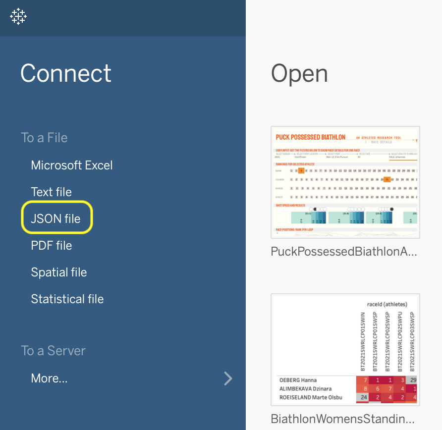
Football and baseball are huge sports in the fantasy sports world. Biathlon is not, however that doesn’t mean it is not there at all. For example, the sports department of the German television corporation ARD has what they call the Biathlon Tipp Spiel, freely translated as the biathlon guessing game. It allows participants to predict the top 5 of any upcoming race in the IBU World Cup circuit, and although thankfully biathlon is unpredictable enough to make this pretty hard, I wanted to have a quick look into previous results to see “who’s hot and who’s not”. The following blog-post describes the steps I took to create the Puck Possessed Biathlon Athletes Research Tool on Tableau Public. For those of you who eagerly clicked on the link, please be patient as the data loads 3+ season of detailed race results. Update: I created a clone that eliminates the 2017-2018 season, resulting in better performance of the dashboards.

The data

Since the Real Biathlon data is now available through Patreon, I downloaded some of the more current race results using R. Now, there are many other coding languages and ways to do it, but since I’m most familiar with R, that is what I used. The following paragraph is a description of how the get the data using R (assuming you have a subscription). If you’re not interested in the technical stuff, skip right ahead to the Data Visualization section below.

First we need to connect to the Mongo Data base with the username and password that comes with the Patreon subscription:

install.packages("mongolite", "tidyverse", "dplyr", "jsonlite")
library(mongolite)
library(dplyr)
library(tidyverse)
library(jsonlite)

# Set username and pasword
mongousr <- "--your username--"
mongopw <- "--your password--"

# Set the collection, database and prefix to create the url
rbcol <- "Races"
rbdb <- "Results"
rbpref <- "biathloncluster-ay3ak"
rburl <- paste("mongodb+srv://",mongousr,":",mongopw,"@",rbpref,".mongodb.net/<dbname>?retryWrites=true&w=majority", sep="")

# Use the URL created above to connect to the correct MongoDB data
rbmongo <- mongo(collection = rbcol, db = rbdb, url = rburl, verbose = TRUE)

Now we can connect to the database. To gather all the data I wanted for my dashboard, I first got data that had all raceIds I wanted to download. Then I created a loop to go through these raceIds one by one and download the file. Below is just the code to get one single file into Tableau. Perhaps I’ll show the loop code in another blog post sometime.

# Get data from the Mongo connection created above by searching for one specific raceId
RaceBT2021SWRLCP01SWSP <- rbmongo$find('{"raceId" : "BT2021SWRLCP01SWSP"}')

# Convert the file to json
RaceBT2021SWRLCP01SWSPjson <- toJSON(RaceBT2021SWRLCP01SWSP)

# Write the json file to your computer
write(RaceBT2021SWRLCP01SWSPjson, "RaceBT2021SWRLCP01SWSPjson.json")

And that is all it takes to connect, load a file and save it as a json file. One could also save as a flat csv file here, but to do that you will have to manipulate the loaded file first as it comes with nested data, multiple levels deep. Since Tableau Public reads json files natively, I decided that using the power of Tableau Public is far more time-efficient.

Data visualization

Although the above code generates one json file for one race, for my specific dashboard I got a file for every race since the 2017-2018 season, creating over 200 files. With those sitting on my hard drive, eagerly awaiting to be visualized, do the following:

Open Tableau Public and connect to a Json file

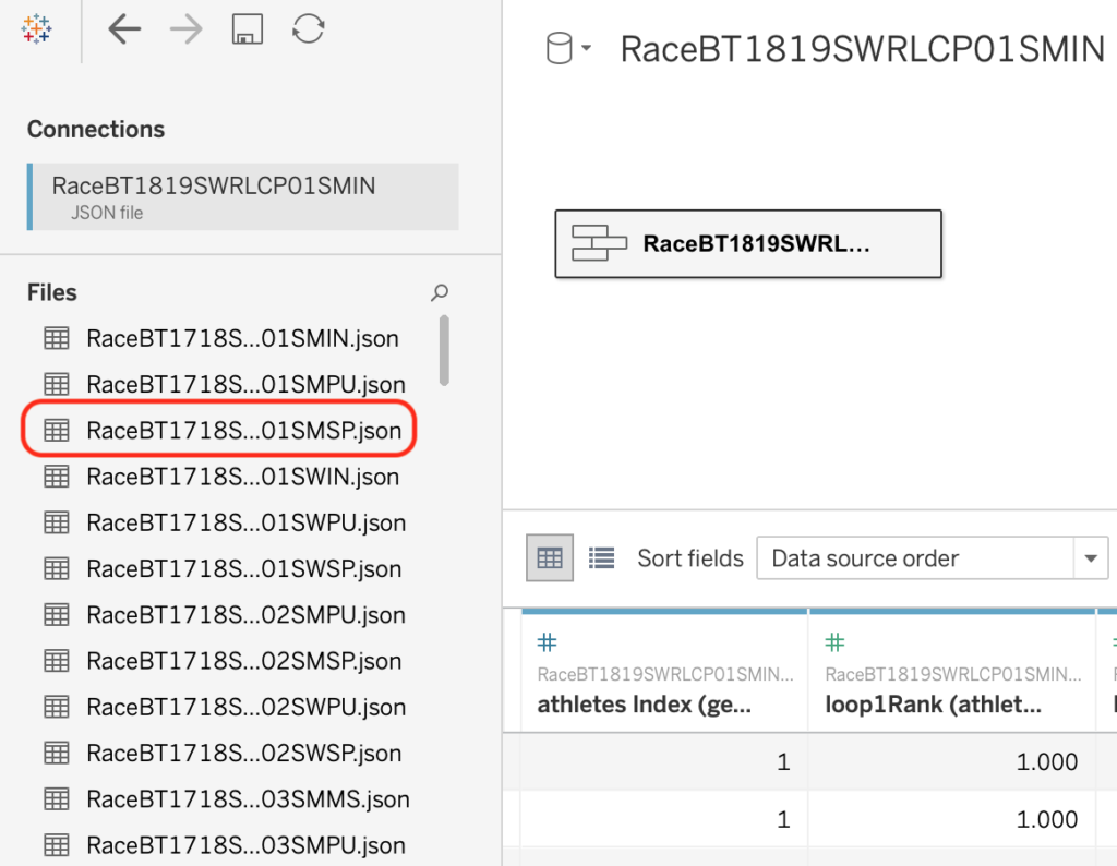
Select one json file specifically

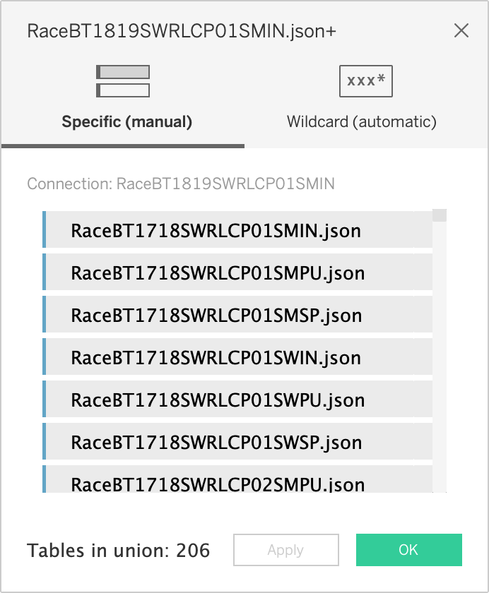
Drag all other json files (I assume all files are in the same folder as the first file) right below the one file from the screenshot above

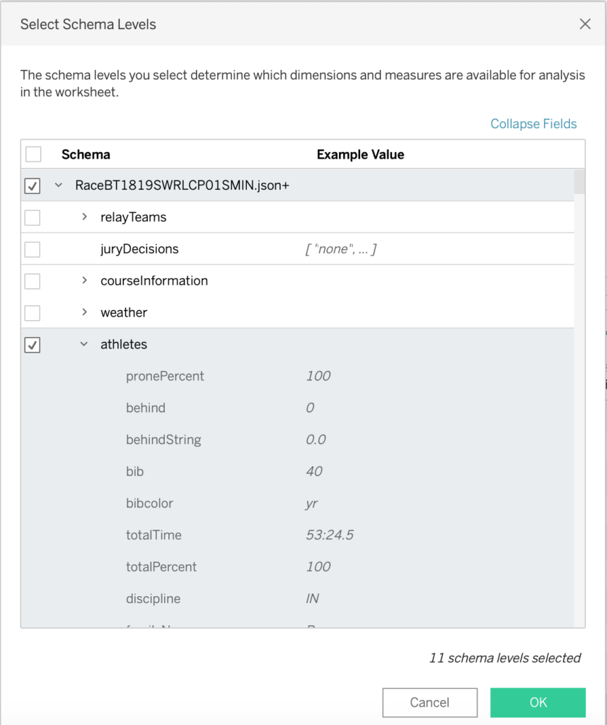
Select the Schema Levels to only get the data I want to use (resist the temptation to select all when you see all the goodness that is available in these files, and stick to the KISS principle)

Now you can create a new Sheet and start on your visualization. I must admit working with the nested json files takes a little time to get used to if you are used to dealing with flat files, but in the end it works quite well!


Since I wanted to have information on athletes specifically to help me pick future winners, I wanted to make three levels of information, or dashboards: one for one race, specifically the most recent one or the most recent of the same type and on the same location as the one I’m predicting for, one to show me current form by looking at the results for the current season to date, and one for similar events in the past (so all sprint races in the last couple of seasons, or all races in Hochfilzen, etc.)

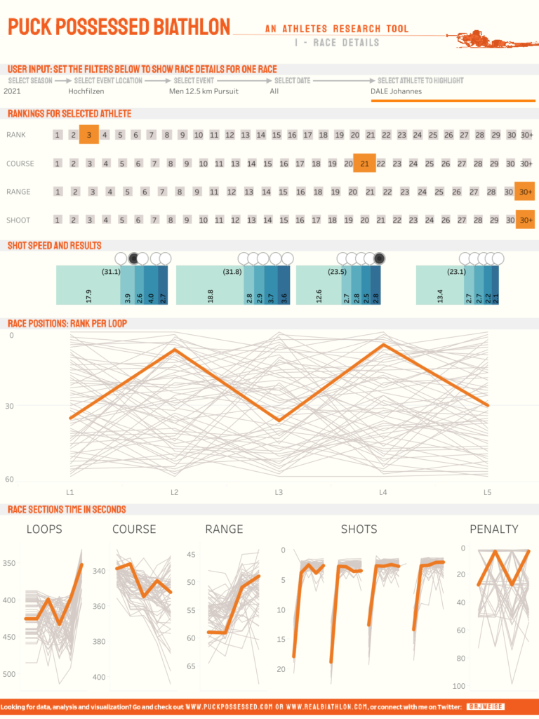
Tab 1 Race Details shows infomartion for one race, while highlighting one athlete of choice

Tab 2 Current Season Information shows information about the selected athlete that gives the reader an idea if the athlete is hot or not, or on an upward or downward trend.

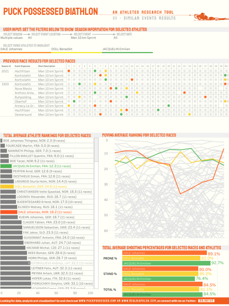
Tab 3 Similar Events Results shows how athletes have performed in previous similar races as the one you are predicting for.

So please go have a look at the dashboards (full and small) and let me know what you think. And good luck making your own dashboards based on the real biathlon Patreon data subscription!

Posted in Statistical analysis | Tagged Data subscription, data visualization, Patreon, R, Tableau

Improvements season-to-season, putting it to use

Posted on 2020-11-19 | by biathlonanalytics | 2 Comments on Improvements season-to-season, putting it to use

To highlight what a great site Real biathlon is, and how easily the data can be used to give some great insights, below is a step-by-step on how to make a quick interactive chart based on the data referenced in the previous article. I used Google Sheets and Tableau Public, but you can use any of these kinds of tools that you are comfortable with, and publish a lookup chart within an hour. That’s how easy the real biathlon site is to collect biathlon data!

Step 1 – download & store the data

For the created chart I used the data of the last five season, for both men and women, limiting the data to only those athletes with at least 10 races. Since that never resulted in more than 100 athletes per gender and season, I did not set a filter on that.

After selecting the Season Statistics, Performance Score (for example, the 2019-2020 season for women), you can just select the table, copy, open a blank Google Sheet, select cell A1 and paste. In my case, my first row showed twice so I just removed one of them. Do this 10 times (five per gender), name the sheets appropriately (W1920, W1819, M1920, M1819, etc.) and export from Google Sheets to an xlsx file. You can export to text, but you would have to do that per sheet, where exporting to excel (xlsx) exports all sheets at once.

Step 2 – open data in Tableau

In Tableau Public connect to the spreadsheet by:

  • clicking on the Data menu > New Data Source
  • click on Microsoft Excel in the Connect window
  • select the xlsx file you just exported from Google Sheets
  • at the bottom of the list that shows your sheet names, double click New Union
  • drag all 10 sheets into the Union window
  • click OK

Step 3 – create some calculated fields

  • Full Name = [Given Name] + ” ” + [Family Name]
  • Gender =
IF LEFT([Table Name],1) = "M" THEN "Men"
ELSEIF LEFT([Table Name],1) = "W" THEN "Women"
ELSE "Unknown"
END
  • Season = MID([Table Name],2,5)

Step 4 – create the chart

Depending on what you want to show in your chart, the following differs, but to replicate the chart I made, drag the following pills in the Filters, Marks, Columns and Rows:

Step 5 – publish to Tableau Public

Once you are happy with your chart, just save the file to Tableau Public.

Now users can use highlighters to see how their favourite athletes stack up against the field, or see how certain Nations fare.

Posted in Statistical analysis | Tagged data use examples, data visualization, Tableau

Recent Articles

  • Most improved athletes this winter
  • New biathlon point system
  • Historic biathlon results create expectations. But what about points?
  • What do you expect? Practical applications of the W.E.I.S.E.
  • Introducing W. E. I. S. E: the Win Expectancy Index based on Statistical Exploration, version 1

Categories

  • Biathlon Media
  • Biathlon News
  • Long-term trends
  • Statistical analysis
  • Website updates

Archives by Month

  • 2022: J F M A M J J A S O N D
  • 2021: J F M A M J J A S O N D
  • 2020: J F M A M J J A S O N D
  • 2015: J F M A M J J A S O N D
  • 2013: J F M A M J J A S O N D
  • 2012: J F M A M J J A S O N D

Search Articles